Chi-Square Test for Feature Selection: A Test Powered By Multinomial Distribution

Feature selection with chi-square looks simple on the surface, yet underneath it lies a multinomial probabilistic structure that most implementations never explain.

Feature selection is a critical component of building a classification model. This phase determines whether useful and informative features are provided to the model. Among the many statistical techniques available, the chi-square test is one of the most widely used methods for feature selection, especially when dealing with categorical data.

In this article, we will understand what the chi-square test is and explore its theoretical foundation to see why it works as a feature selection technique.

At its core, the chi-square test is a non-parametric statistical test that helps identify whether a feature carries discriminatory information about the class label.

It answers a fundamental question:

“Does the feature carry information about the class label, or is it distributed independently of the class label?”

Hypothesis Testing Framework

Before diving into the mathematical foundations, let us understand how the chi-square test is framed as a hypothesis test.

We begin by assuming that the feature and the class label are statistically independent. This forms the null hypothesis. The alternative hypothesis states that the feature and the class label are statistically dependent.

To test this assumption, we collect data and compute a test statistic that compares what we observe in the data with what we would expect to observe if independence were true.

If the difference between the observed behavior and the expected behavior is sufficiently large, we reject the null hypothesis. This implies that the feature and the class label are statistically dependent, and therefore, the feature carries discriminatory power.

It is important to note that the chi-square test applies only to categorical variables. If a variable is continuous, it must first be discretized into bins. The chi-square statistic then measures how observed counts across these bins deviate from expected counts under independence.

This naturally raises an important question:

How is the expected behavior defined, and why do large deviations imply dependence?

To answer this, we need to understand the probabilistic foundation of the test.

Multinomial Distribution

The journey of the chi-square test begins with the multinomial distribution.

The multinomial distribution is a generalization of the binomial distribution to more than two outcomes. Suppose we conduct an experiment with N trials. In each trial, exactly one outcome is observed, chosen from K possible outcomes, where K > 2.

Over N trials, the number of times each outcome occurs follows a multinomial distribution.

The probability mass function of multinomial distribution is given as follows:

\(P(X_1 = x_1, X_2 = x_2, ..., X_K = x_K) = \frac{N!}{x_1! x_2! \cdots x_K!} \prod_{k=1}^{K} p_k^{x_k} \)

where,

\(\sum_{k=1}^{K} x_k = N \quad \text{and} \quad \sum_{k=1}^{K} p_k = 1 \)

Let us understand this with a banking example.

Consider a bank that observes 10,000 transactions on a given day. Transactions are processed through four channels: cash, wire, ATM, and online payment.

Each transaction represents one trial, and each trial results in exactly one channel. A transaction cannot belong to more than one channel.

Let:

• X1 = number of cash transactions

• X2 = number of wire transactions

• X3 = number of ATM transactions

• X4 = number of online transactions

Let N = 10,000 denote the total number of transactions.

Then the joint distribution of (X1, X2, X3, X4 ) follows a multinomial distribution. This allows us to compute probabilities such as observing 200 cash transactions, 6,000 wire transactions, 2,000 ATM transactions, and 1,800 online transactions on a given day.

Now, let us extend this idea to two categorical variables, which is exactly the setting required for the chi-square test.

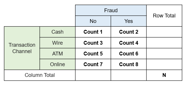
Contingency Table

When two categorical variables are involved, their joint behavior is conveniently represented using a contingency table.

In our case:

• Variable 1: Transaction channel

• Variable 2: Fraud status (Yes / No)

A contingency table does more than just summarize data. Each cell in the table represents a random variable, and the counts across all cells jointly follow a multinomial distribution.

This is because:

• Each transaction belongs to exactly one combination of channel and fraud status.

• The total number of transactions is fixed.

Since we have four transaction channels and two fraud outcomes, there are ( 4*2 = 8 ) possible combinations:

• (Cash, No), (Cash, Yes)

• (Wire, No), (Wire, Yes)

• (ATM, No), (ATM, Yes)

• (Online, No), (Online, Yes)

Each of these combinations corresponds to one cell in a (4*2) contingency table

When we observe the data for a given day, the contingency table we construct is one realization of an underlying multinomial process. In other words, the observed table is generated by a probabilistic mechanism governed by multinomial probabilities.

Independence Assumption

Let us now connect this setup to the hypothesis of independence.

Consider a general contingency table with r rows and c columns. Let (Pij) denote the probability that an observation falls into cell (i,j).

Under the null hypothesis of independence:

\(P_{ij} = P_{i\cdot} \times P_{\cdot j}\)

This means that the probability of an observation falling into a particular cell depends only on the marginal probabilities of the row and the column, and not on any interaction between them.

In simple terms, in our banking example, this implies that fraud status does not depend on the transaction channel.

Observed vs Expected Table

So far, we have discussed probabilities. In practice, however, we observe counts, not probabilities.

For example, the cash channel may show 100 fraudulent transactions and 500 non-fraudulent transactions. These are observed counts.

To perform the chi-square test, we need to determine what the counts would look like if the independence assumption were true.

This is done by constructing an expected contingency table under independence.

Under this assumption, knowing the row totals (transaction channel distribution) and column totals (fraud distribution) is sufficient to reconstruct the entire table.

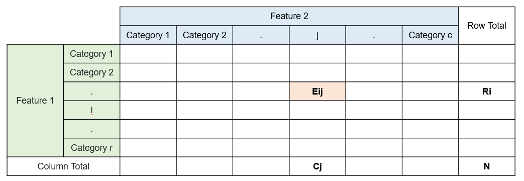
The expected count in cell (i,j) is given by:

\(E_{ij} = \frac{R_i \times C_j}{N}\)

where:

• Ri is the total count in row i

• Cj is the total count in column j

• N is the total number of observations

This formula arises directly from the multinomial distribution combined with the independence assumption. If the observed counts closely match the expected counts, independence is plausible. Large deviations indicate interaction between the variables.

Quick Derivation for Expected Count

Under the null hypothesis of independence,

\(\begin{aligned} P_{ij} &= P(X = i, Y = j) \\ &= P(X = i)\,P(Y = j) \\ \end{aligned}\)

The marginal probabilities are estimated from observed data as

\(P(X = i) = R_i / N\)

\(P(Y = j) = C_j / N\)

Substituting these into the independence assumption,

\(P_{ij} = (R_i / N) × (C_j / N)\)

Using the multinomial distribution assumption, the expected count in cell (i, j) is defined as

\(E_{ij} = N × P_{ij}\)

Substituting the expression for Pij

\(E_{ij} = N × ((R_i / N) × (C_j / N))\)

Simplifying,

\(E_{ij} = (R_i × C_j) / N\)

Test Statistic Derivation

Once the expected counts are computed, the next step is to quantify how far the observed data deviates from the expected behavior.

For a given cell (i,j), the raw deviation is:

\(O_{ij} - E_{ij}\)

However, each cell count is a random variable with natural variability. To compare deviations across cells meaningfully, we must scale the difference by the variability of the cell count.

The standardized deviation is defined as:

\(\frac{O_{ij} - E_{ij}}{\sqrt{E_{ij}}}\)

Under the null hypothesis, this standardized quantity approximately follows a standard normal distribution.

To avoid cancellation between positive and negative deviations, we square each standardized deviation and sum across all cells:

\(\chi^2 = \sum_{i=1}^{r} \sum_{j=1}^{c} \frac{(O_{ij} - E_{ij})^2}{E_{ij}}\)

From statistical theory, the sum of squared standard normal variables follows a chi-square distribution. The resulting test statistic follows a chi-square distribution with (r-1)*(c-1) degrees of freedom.

A small value of the test statistic supports independence. A large value provides evidence against independence, indicating that the feature carries discriminatory information and is useful for feature selection.

The final decision is made by comparing the test statistic with the chi-square distribution at a chosen significance level.